I can never remember the difference between left and right multiplying transform matrices, so I’m writing all this down mostly for myself.
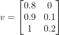
Let ![]() be an array of 2D vectors of
shape
be an array of 2D vectors of
shape ![]() :
:

Let ![]() be a
be a ![]() degrees counterclockwise
rotation matrix:
degrees counterclockwise
rotation matrix:
![]()
Expressed with a right multiply, the rotated ![]() would be
would be
![]()
Note the shapes: ![]() is
is ![]() and
and ![]() is
is ![]() , so we end up
with
, so we end up
with ![]() . In numpy for a 30 degree counterclockwise
rotation:
. In numpy for a 30 degree counterclockwise
rotation:
v = np.array([[0.8, 0], [0.9, 0.1], [1, 0.2]])

def make_rotation_matrix(K_rad):
    return np.array([[np.cos(K_rad), -np.sin(K_rad)],
                     [np.sin(K_rad), np.cos(K_rad)]])

vprime = (make_rotation_matrix(np.deg2rad(30)) @ v.T).T
which, visualized as vectors from the origin, produces the expected result:

Expressed with a left multiply, the rotated ![]() would be
would be
![]()
Note the shapes: ![]() is
is ![]() and
and ![]() is
is ![]() , so we end up
with
, so we end up
with ![]() . In
numpy:
. In
numpy:
vprime = v @ make_rotation_matrix(np.deg2rad(30)).Twhich again visualized as vectors from the origin produces the same result:

Imagine instead of a simple rotation by ![]() , we also wanted to transform
the points that included a translation
, we also wanted to transform
the points that included a translation ![]() . We
could represent this as two separate operations, a rotation and a
translation, or we could represent it as a single homogeneous transform
. We
could represent this as two separate operations, a rotation and a
translation, or we could represent it as a single homogeneous transform
![]() :
:
![]()
where ![]() is the same rotation matrix as
before, and
is the same rotation matrix as
before, and ![]() is the column version of the
translation vector (i.e.
is the column version of the
translation vector (i.e. ![]() ). To do this, we augment
the
). To do this, we augment
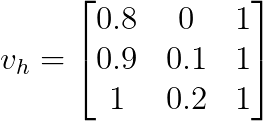
the ![]() vectors with a third column of
ones, i.e.
vectors with a third column of
ones, i.e.

making it an ![]() matrix. The
homogeneous transform
matrix. The
homogeneous transform ![]() is a
is a ![]() matrix, so we
can left multiply it with
matrix, so we
can left multiply it with ![]() to get the transformed
to get the transformed ![]() :
:
![]()
In numpy
def make_transform_matrix(K_rad, translation):
    return np.array([[np.cos(K_rad), -np.sin(K_rad), translation[0]],
                     [np.sin(K_rad), np.cos(K_rad), translation[1]],
                     [0, 0, 1]])

def make_homogeneous(v):
    return np.hstack((v, np.ones((v.shape[0], 1))))

vprime_h = v_h @ make_transform_matrix(rotation, translation).T
which, visualized as vectors from the origin, produces the expected result:
